44 add data labels to pivot chart
Add Value Label to Pivot Chart Displayed as Percentage ... I have created a pivot chart that "Shows Values As" % of Row Total. This chart displays items that are On-Time vs. items that are Late per month. The chart is a 100% stacked bar. I would like to add data labels for the actual value. Example: If the chart displays 25% late and 75% on-time, I would like to display the values behind those %'s, such as 1 late and 3 on-time. Pivot Chart data labels - Excel Help Forum For a new thread (1st post), scroll to Manage Attachments, otherwise scroll down to GO ADVANCED, click, and then scroll down to MANAGE ATTACHMENTS and click again. Now follow the instructions at the top of that screen. New Notice for experts and gurus:
How to add and customize chart data labels - Get Digital Help The image above demonstrates data labels in a line chart, each data point in the chart series has a visible data label. Edit data labels. Excel allows you to edit the data label value manually, simply press with left mouse button on a data label until it is selected.

Add data labels to pivot chart
Add or remove data labels in a chart - support.microsoft.com Add data labels to a chart Click the data series or chart. To label one data point, after clicking the series, click that data point. In the upper right corner, next to the chart, click Add Chart Element > Data Labels. To change the location, click the arrow, and choose an option. If you want to ... Create Dynamic Chart Data Labels with Slicers - Excel Campus You basically need to select a label series, then press the Value from Cells button in the Format Data Labels menu. Then select the range that contains the metrics for that series. Click to Enlarge Repeat this step for each series in the chart. If you are using Excel 2010 or earlier the chart will look like the following when you open the file. Changing data label format for all series in a pivot chart ... To change data labels format, please perform the following steps: Click the pivot chart > + sign near tthe pivot chart > right click data label of any series > Format Data Series... Besides, to move forward, could you please provide the following information? 1. Do all series have data labels when you create a pivot chart?
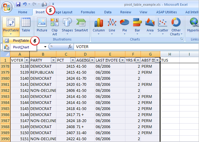
Add data labels to pivot chart. Custom data labels in a chart - Get Digital Help If you have excel 2013 you can use custom data labels on a scatter chart. 1. Right press with mouse on a series 2. Press with left mouse button on "Add Data Labels" 3. Right press with mouse again on a series 4. Press with left mouse button on "Format Data Labels" 5. Enable check box "Value from cells" 6. Select a cell range 7. Disable check box "Y Value" How to add data labels from different column in an Excel ... Please do as follows: 1. Right click the data series in the chart, and select Add Data Labels > Add Data Labels from the context menu to add... 2. Right click the data series, and select Format Data Labels from the context menu. 3. In the Format Data Labels pane, under Label Options tab, check the ... Pivot Table Tip- Assign The Correct Row And Column Labels ... The first thing to do is put your cursor somewhere in your data list. Select the Insert Tab. Hit Pivot Table icon. Next select Pivot Table option. Select a table or range option. Select to put your Table on a New Worksheet or on the current one, for this tutorial select the first option. Click Ok. The Options and Design Tab will appear under ... How to add data labels to pivot chart? | Console App ... The CSV data goes into the Data sheet and the application then creates a pivot table and corresponding pivot chart from this data in the Charts sheet. The chart is created alright but i see no option to add data labels to it using XlsIO. The chart is created as follows: IChartShape pivotChart = chartsSheet.Charts.Add();
Multiple Data Labels on bar chart? - Excel Help Forum Apply data labels to series 1 inside end. Select A1:D4 and insert a bar chart. Select 2 series and delete it. Select 2 series, % diff base line, and move to secondary axis. Adjust series 2 data references, Value from B2:D2. Category labels from B4:D4. Apply data labels to series 2 outside end. select outside end data labels and change from ... How to Add Data Labels to an Excel 2010 Chart - dummies On the Chart Tools Layout tab, click Data Labels→More Data Label Options. The Format Data Labels dialog box appears. You can use the options on the Label Options, Number, Fill, Border Color, Border Styles, Shadow, Glow and Soft Edges, 3-D Format, and Alignment tabs to customize the appearance and position of the data labels. How to Customize Your Excel Pivot Chart Data Labels - dummies To add data labels, just select the command that corresponds to the location you want. To remove the labels, select the None command. If you want to specify what Excel should use for the data label, choose the More Data Labels Options command from the Data Labels menu. Excel displays the Format Data Labels pane. How to create Custom Data Labels in Excel Charts Create the chart as usual. Add default data labels. Click on each unwanted label (using slow double click) and delete it. Select each item where you want the custom label one at a time. Press F2 to move focus to the Formula editing box. Type the equal to sign. Now click on the cell which contains the appropriate label.
Add a data label on Pivot Chart With .SeriesCollection (1).Points (i) .HasDataLabel = True .DataLabel.Text = Worksheets ("Sheet2").Range ("a" & position_total).Value position_total = position_total + 1 End With End With Next End Sub Select the Pivot chart, then run the macro "data_label". Jaynet Zhang TechNet Community Support How to add Data label in Stacked column chart of Pivot charts I'm tring to make a Pivot chart with stacked column graph. In where, i couldn't add data label for cumulative sum of value in Data label. Where i could only add data label to individual stacks in column graph. It found possible with normal stacked column chart without pivot chart. Can someone please help me to resolve this? Add a Data Callout Label to Charts in Excel 2013 ... The new Data Callout Labels make it easier to show the details about the data series or its individual data points in a clear and easy to read format. How to Add a Data Callout Label. Click on the data series or chart. In the upper right corner, next to your chart, click the Chart Elements button (plus sign), and then click Data Labels. Formal ALL data labels in a pivot chart at once ... However, you may change the location of the data labels all at once, as you can see in screenshot below: I would suggest you vote for or leave your comments in the thread: Format Data Labels (Ex: Alignment/Text Direction) of Multiple Data Series together in Excel UserVoice to let the related team of Office hear your Voice, which will promote them to develop the related feature in Excel.

How to Create Multi-Category Chart in Excel - Excel Board
How to add data label value in bar chart in python pivot ... import pandas as pd import numpy as np import matplotlib.pyplot as plt employees = {'Name of Employee': ['Jon','Mark','Tina','Maria','Bill','Jon','Mark','Tina','Maria ...
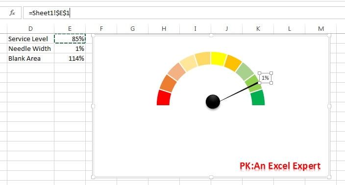
Speedometer Chart - PK: An Excel Expert
Change the format of data labels in a chart To format data labels, select your chart, and then in the Chart Design tab, click Add Chart Element > Data Labels > More Data Label Options. Click Label Options and under Label Contains, pick the options you want. To make data labels easier to read, you can move them inside the data points or even outside of the chart.

excel - remove data labels automatically for new columns in pivot chart? - Stack Overflow
Add Data Bar To Labels Chart Matplotlib Search: Matplotlib Add Data Labels To Bar Chart. Let's see how many numbers are between -10 and -1, between -1 and 1, and between 1 and 10 One axis The bars can be plotted vertically or horizontally 0 that's causing tick labels for logarithmic axes to revert to the default font Add and modify chart value labels Add and modify chart value labels.

31 Excel Chart Label Axis - Label Design Ideas 2020
Custom Chart Data Labels In Excel With Formulas Select the chart label you want to change. In the formula-bar hit = (equals), select the cell reference containing your chart label's data. In this case, the first label is in cell E2. Finally, repeat for all your chart laebls. If you are looking for a way to add custom data labels on your Excel chart, then this blog post is perfect for you.

WinForms Pivot Chart Control | Business Charts | Syncfusion
How to Add Data Labels in Excel - Excelchat | Excelchat In Excel 2013 and the later versions we need to do the followings; Click anywhere in the chart area to display the Chart Elements button Figure 5. Chart Elements Button Click the Chart Elements button > Select the Data Labels, then click the Arrow to choose the data labels position. Figure 6. How to Add Data Labels in Excel 2013 Figure 7.

Did you know: Multiple Pivot Charts for the SAME pivot table? - Efficiency 365
How to Add Data to a Pivot Table in Excel | Excelchat We can Add data to a PivotTable in excel with the Change data source option. "Change data source" is located in "Options" or "Analyze" depending on our version of Excel. The steps below will walk through the process of Adding Data to a Pivot Table in Excel. Figure 1- How to Add Data to a Pivot Table in Excel. Setting up the Data

excel - How can I incorporate a PivotTable right into the source data on the sheet (using EPPlus ...
Add data labels, notes, or error bars to a chart ... Double-click the chart you want to change. At the right, click Customize Series. Check the box next to "Data labels." Tip: Under "Position," you can choose if you want the data label to be inside...
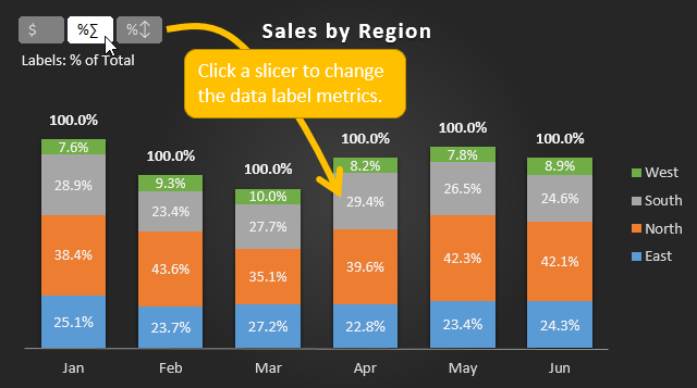
Create Dynamic Chart Data Labels with Slicers - Excel Campus
How to change/edit Pivot Chart's data source/axis/legends ... Step 1: Select the Pivot Chart you will change its data source, and cut it with pressing the Ctrl + X keys simultaneously. Step 2: Create a new workbook with pressing the Ctrl + N keys at the same time, and then paste the cut Pivot Chart into this new workbook with pressing Ctrl + V keys at the same time.

excel vba - VBA Pivot Chart data labels not appear - Stack Overflow
Adding rich data labels to charts in Excel 2013 ... To add a data label in a shape, select the data point of interest, then right-click it to pull up the context menu. Click Add Data Label, then click Add Data Callout . The result is that your data label will appear in a graphical callout. In this case, the category Thr for the particular data label is automatically added to the callout too.

How to Sort Pivot Table Row Labels, Column Field Labels and Data Values with Excel VBA Macro ...
Changing data label format for all series in a pivot chart ... To change data labels format, please perform the following steps: Click the pivot chart > + sign near tthe pivot chart > right click data label of any series > Format Data Series... Besides, to move forward, could you please provide the following information? 1. Do all series have data labels when you create a pivot chart?
In Search of the Elusive Pivot Table | Dynamic Edge, Inc. | Beyond Tech Support Dynamic Edge ...
Create Dynamic Chart Data Labels with Slicers - Excel Campus You basically need to select a label series, then press the Value from Cells button in the Format Data Labels menu. Then select the range that contains the metrics for that series. Click to Enlarge Repeat this step for each series in the chart. If you are using Excel 2010 or earlier the chart will look like the following when you open the file.
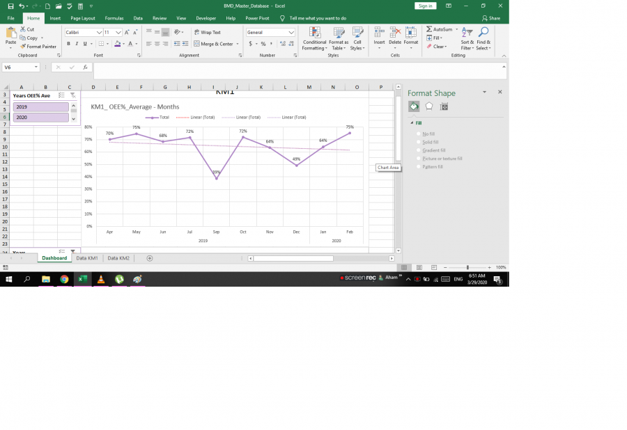
How to add the average baseline for a specific pivot chart | Dashboards & Charts | Excel Forum ...
Add or remove data labels in a chart - support.microsoft.com Add data labels to a chart Click the data series or chart. To label one data point, after clicking the series, click that data point. In the upper right corner, next to the chart, click Add Chart Element > Data Labels. To change the location, click the arrow, and choose an option. If you want to ...

vba - Pie Chart - Move Data Labels off Chart - Stack Overflow
Sort data in a PivotTable or PivotChart
Post a Comment for "44 add data labels to pivot chart"